Evaluations

METRICS

We propose a total of 15 accuracy, realism, and decidability metrics. These metrics are either borrowed from computer vision and computer graphics literature or newly developed multiverse metrics, which assess the A2A and A2E interactions of both multimodal models with k >1 and unimodal models with k= 1.

Accuracy Metrics: Comparison to Ground Truth

Accuracy metrics from computer vision literature are responsible for comparing the ground truth with the predictions based on the displacement error.

Metric	Description
Average Displacement Error (ADE)	ADE is computed for each prediction \( j \) as \( a_j \), the average distance between a position in the ground truth and a position in the prediction across \( t_f \) frames. It is then aggregated across the \( k \) predictions in three ways: minimum, mean, and maximum, which offers a more reliable expectation of a model’s accuracy than the minimum alone.
Final Displacement Error (FDE)	FDE is computed for each prediction \( j \) as \( b_j \), the distance between the final positions of the ground truth and the prediction. It is aggregated across the \( k \) predictions in the same ways as ADE for better reliability.

Realism Metrics: Motion and Interaction Statistics

Realism metrics are used to describe the movement and interactions within the ground truth and the predictions separately. These metrics can then be used to uncover more nuanced differences between the ground truth and predictions. While they cannot ensure that predictions are accurate, they can ensure that predictions are realistic in their movement and plausible. Every realism metric is computed in the same way for both the ground truth and predictions. For generality, we consider the ground truth as a unimodal model with \( k = 1 \), but we refer to it as having \( k \) paths instead of predictions.

The following motion statistics are used to describe the movement of agent \( a \) in either the ground truth or averaged across the \( k \) predictions. They have been used to evaluate crowd simulations in computer graphics research, but have not yet been used to evaluate predictive models in computer vision.

Metric	Description
Path Length	The average path length (m) for an agent \( a \) is computed by first finding the length of each path \( j \) and then averaging the values across all \( k \) paths.
Speed	In order to report the speed (m/s), the magnitudes \( S \) of velocities in \( V_a \) are first computed for each agent \( a \). Next, two values are reported for speed: the mean speed averaged across \( k \) paths and the maximum speed averaged across \( k \) paths. For each path \( j \) of agent \( a \), the mean and maximum speed are computed across \( t_f - 1 \) frames.
Acceleration Magnitude	Similar to speed, we first compute the magnitudes \( A \) of the difference between every pair of consecutive velocities in \( V_a \) for each agent \( a\). The acceleration magnitude (m/s2) \( A(V_a) \) is then reported in the same way as speed: the mean acceleration magnitude averaged across \( k \) paths and the maximum magnitude averaged across \( k \) paths. Traditional measures of collision are unsuitable for multimodal models in which an agent \( a \) may be colliding with agent \( b \) when it takes the direction of path \( j \), but not when it takes the direction of path \( j + 1 \). We therefore propose multiverse metrics such as Agent Collision-Free Likelihood (ACFL) and Environment Collision-Free Likelihood (ECFL) to measure the A2A and A2E interactions of multimodal models respectively.
Agent Collision-Free Likelihood (ACFL)	In order to assess the quality of A2A interaction under the \( k^{(n - 1)} \) possible futures for \( n \) agents, we propose ACFL, which computes the probability that agent \( a \) has a path that is free of collision in all of the \( k^{(n - 1)} \) possible futures with other agents. The indicator function \( 1_{(R > 0)} \) returns \( 1 \) when the distance between agents \( a \) and \( b \) is greater than \( r \) meters at time \( t \), and \( 0 \) otherwise. This means that if their centers of mass are within \( r \) meters of each other, they are considered to be colliding. For analysis, \( r \) has been set to \( 0.3 \) meters (∼1 foot).
Environment Collision-Free Likelihood (ECFL)	ECFL complements ACFL in that it measures the quality of A2E interaction under the \( k \) possible futures that agent \( a \) can interact with the environment. Namely, it reports the probability that agent \( a \) has a path that is free of collision with the environment. The environment is represented by a binary matrix \( E \), in which each cell corresponds to a square space and is equal to \( 1 \) if that space is navigable and \( 0 \) otherwise. \( E \)[0,0] is aligned with the origin of the position data \( Y \), but \( E \) has a scale of 1/s meters per unit as opposed to \( 1 \) meter per unit like \( Y \). When agent \( a \)’s center of mass is intersecting a non-navigable region of the environment like a wall, the agent is considered to be colliding with the environment.

Decidability Metric: Certainty in Movement Direction

Decidability is a measure of a model’s uncertainty in the movement direction of agents, and it is not strictly opposite between unimodal and multimodal models. If a multimodal model has low enough uncertainty in an agent’s direction of movement, we consider it to be decidable.

Metric	Description
Multiverse Entropy (MVE)	We compute MVE to measure the decidability for agent \( a \). We first transform each path \( j \) into an average direction vector \( D \) as the vector from the initial position \( Y_{a,j,0} \) to the average position of the \( t_f - 1 \) subsequent points. The average direction vectors \( D \) are then transformed into a probability distribution \( p \) over a vector of \( b \)-many equiangular bins. Finally, the entropy of \( p \) is reported as MVE. High values of ACFL and ECFL are contingent on low MVE (high decidability), because high certainty in the direction that an agent will travel along will cause fewer potential collisions with other agents (ACFL) and the environment (ECFL). For experimental purposes, \( b \) has been set to \( k \), so that MVE is maximized when every prediction is in a different direction.
Comparing Realism Metrics	In order to compare realism metrics between the ground truth and predictions for an agent \( a \), we first compute a feature vector for the ground truth \( F_a \), ECFL(\( Y_a, E) \).

Metric

Description

Multiverse Entropy (MVE)

We compute MVE to measure the decidability for agent \( a \). We first transform each path \( j \) into an average direction vector \( D \) as the vector from the initial position \( Y_{a,j,0} \) to the average position of the \( t_f - 1 \) subsequent points. The average direction vectors \( D \) are then transformed into a probability distribution \( p \) over a vector of \( b \)-many equiangular bins. Finally, the entropy of \( p \) is reported as MVE. High values of ACFL and ECFL are contingent on low MVE (high decidability), because high certainty in the direction that an agent will travel along will cause fewer potential collisions with other agents (ACFL) and the environment (ECFL). For experimental purposes, \( b \) has been set to \( k \), so that MVE is maximized when every prediction is in a different direction.

Comparing Realism Metrics

In order to compare realism metrics between the ground truth and predictions for an agent \( a \), we first compute a feature vector for the ground truth \( F_a \), ECFL(\( Y_a, E) \).

Trained Models

A couple of trained models are available to download. These include models that are trained on A2A datasets, A2E datasets, and both.

Model	Description	Download
PECNet (PECN) for A2A	Training is done on datasets for Agent-to-Agent interactions.	Download
PECNet (PECN) for A2E	Training is done on datasets for Agent-to-Environment interactions.	Download
PECNet (PECN) for Both	Training is done on datasets for both Agent-to-Agent and Agent-to-Environment interactions.	Download
Social GAN (SGAN) for A2A	Training is done on datasets for Agent-to-Agent interactions.	Download
Social GAN (SGAN) for A2E	Training is done on datasets for Agent-to-Environment interactions.	Download
Social GAN (SGAN) for Both	Training is done on datasets for both Agent-to-Agent and Agent-to-Environment interactions.	Download
Trajectron++ (T++) for A2A	Training is done on datasets for Agent-to-Agent interactions.	Download
Trajectron++ (T++) for A2E	Training is done on datasets for Agent-to-Environment interactions.	Download
Trajectron++ (T++) for Both	Training is done on datasets for both Agent-to-Agent and Agent-to-Environment interactions.	Download

Evaluation Scripts

We have provided the evaluation scripts (e.g., ipynb file) to run predictions. You simply need to specify where the prediction outputs are located and where to save analysis result. Please note that the prediction outputs should be saved as Numpy array (npy) and follow the shape e.g., [ agent number, 1+k , 12 , 2 ], where 1 is for ground truth, k is for number of predictions, 12 are the number of frames, and 2 is the x and y positions.

Expand Here for Source Code

Evaluation.ipynb	Download
Sample Predictions	Download
Sample Evaluations	Download
Other Required Files	Download

Note: Make sure to extract Sample Predictions (sample_prediction.zip), Sample Evaluations (sample_evaluation.zip), and Other Required Files (additional_required_files.zip) in the same folder that contains the iPython notebook script (evaluation.ipynb).

Results (Qualitative)

Here we show the predictions and ground truth for nine (9) models tested on multiple scenario.


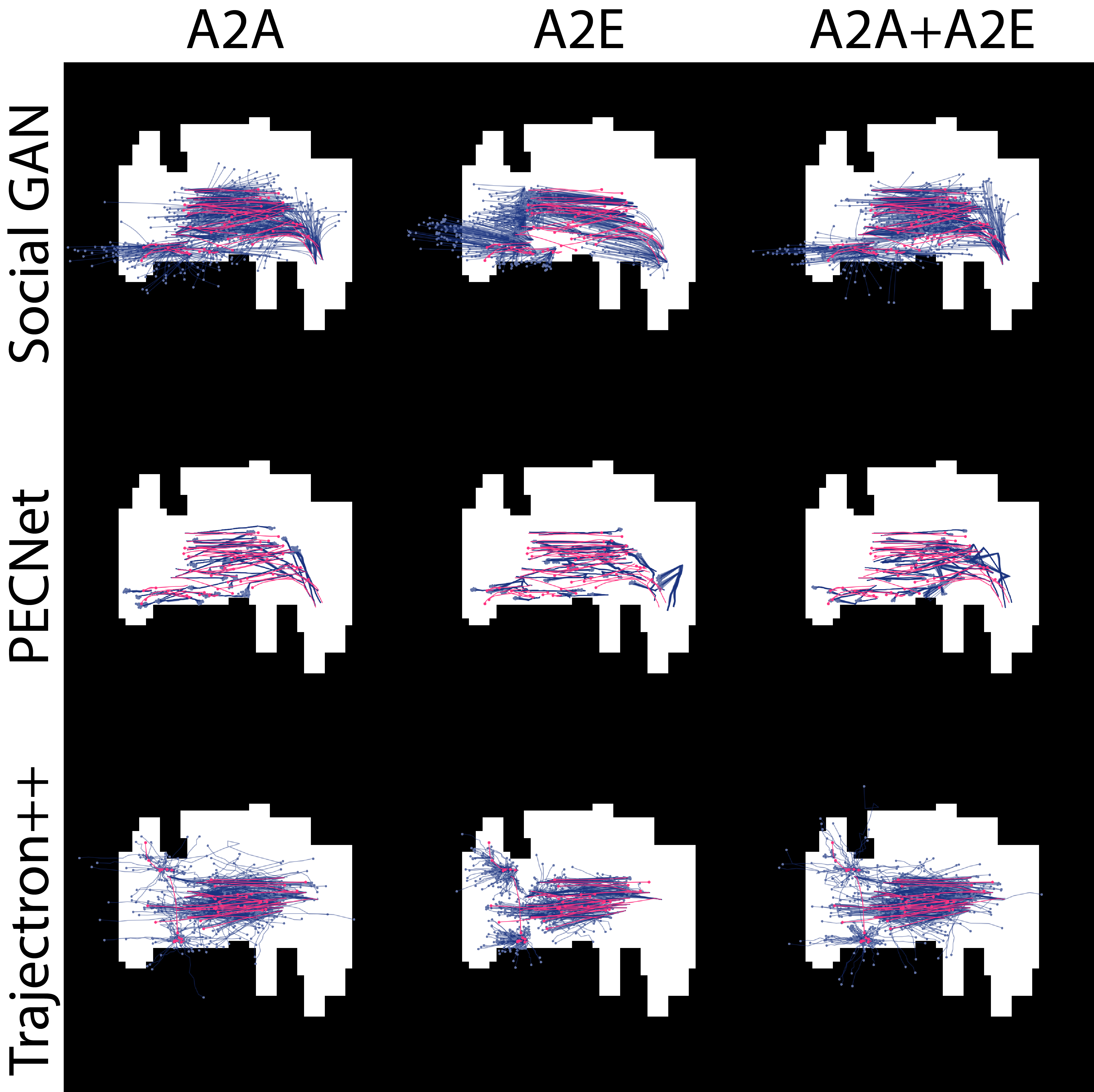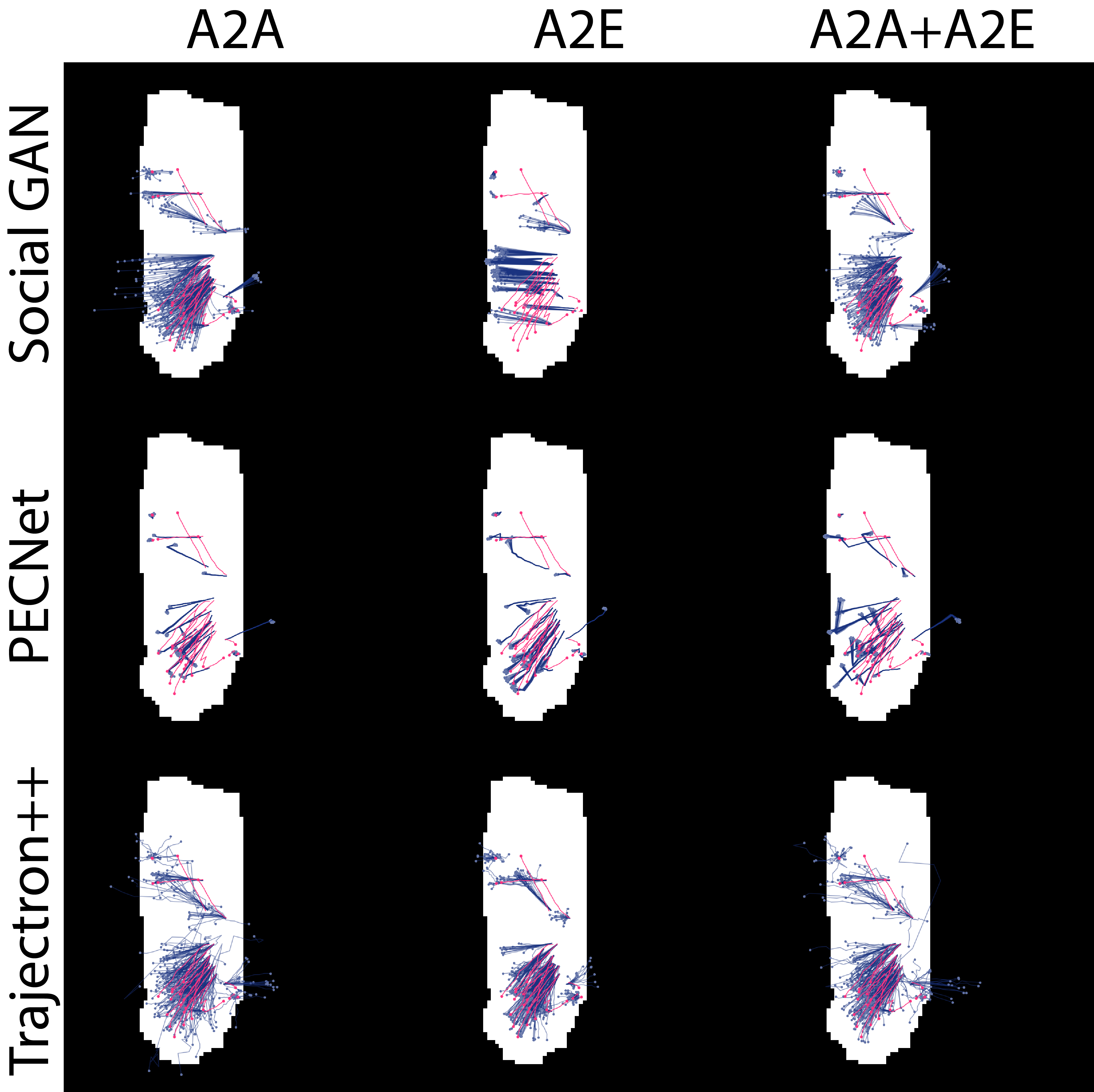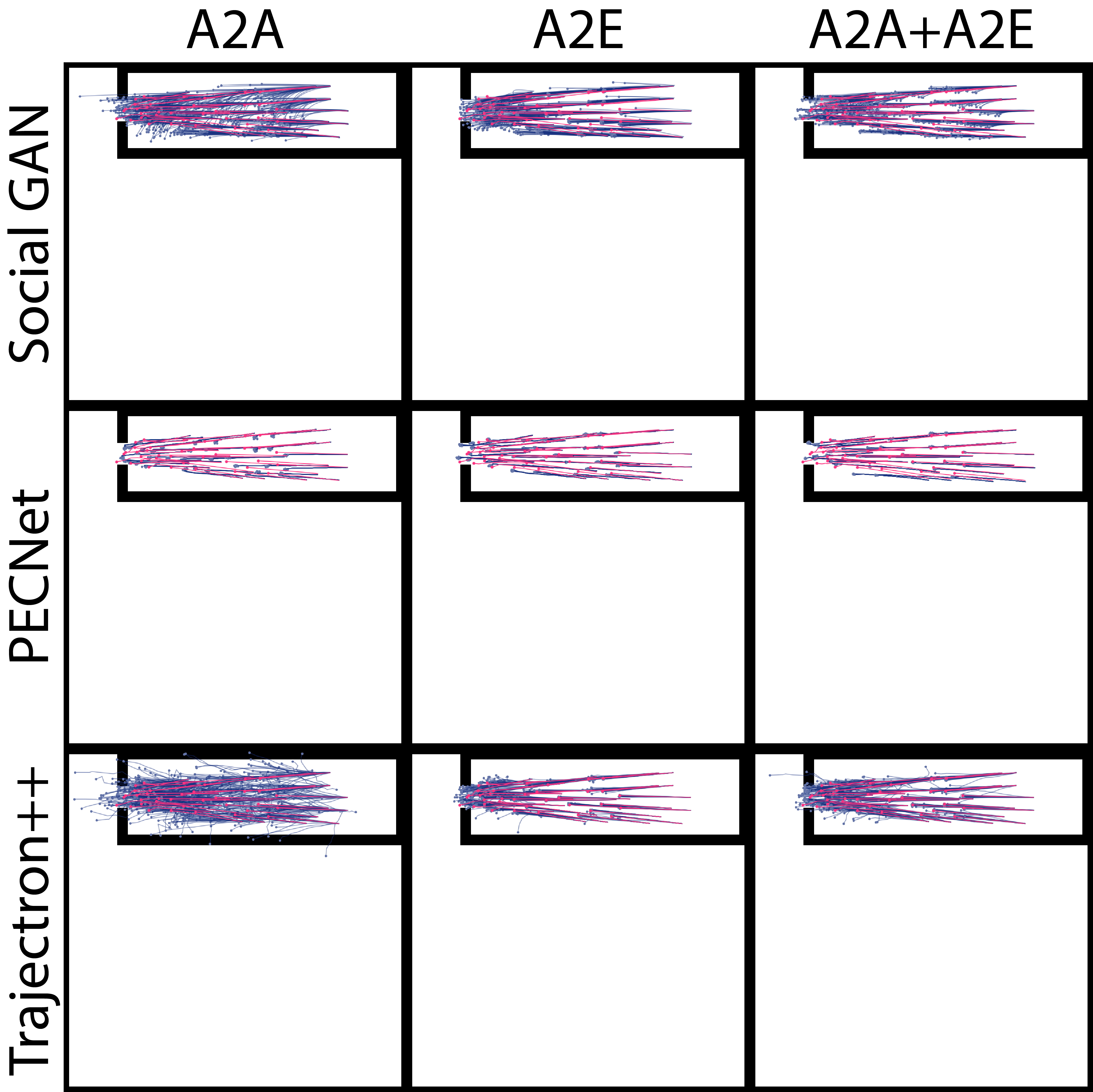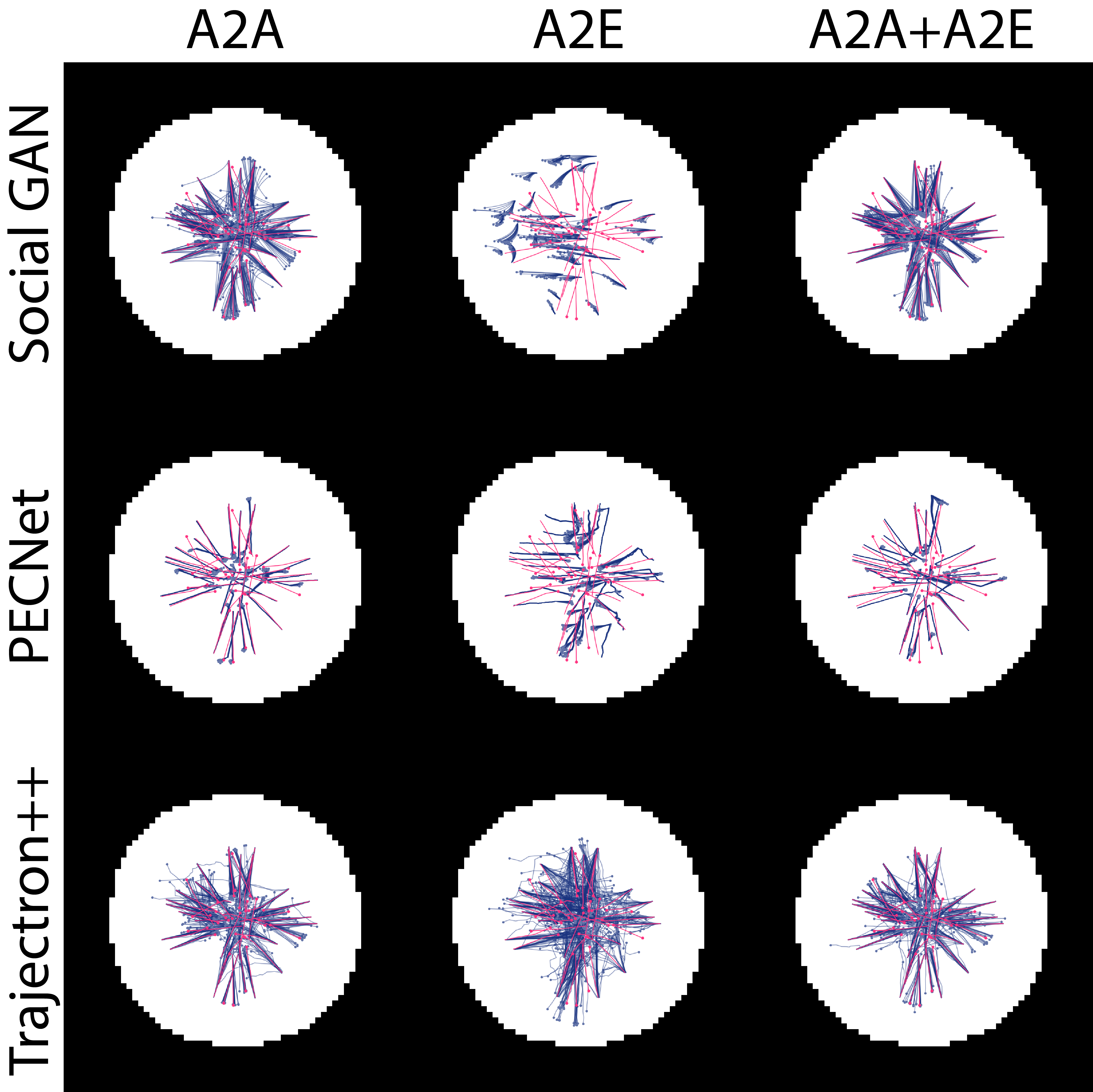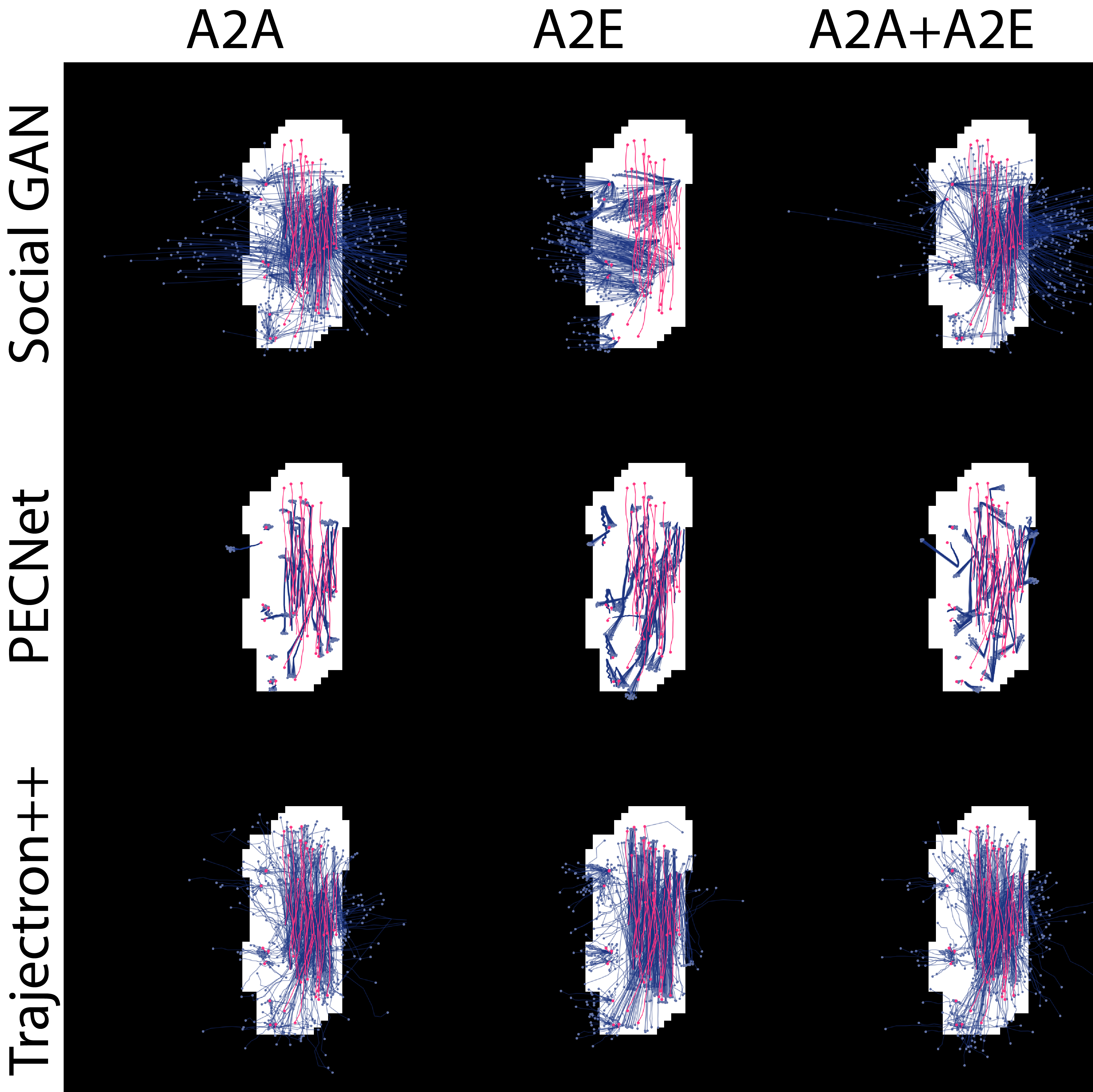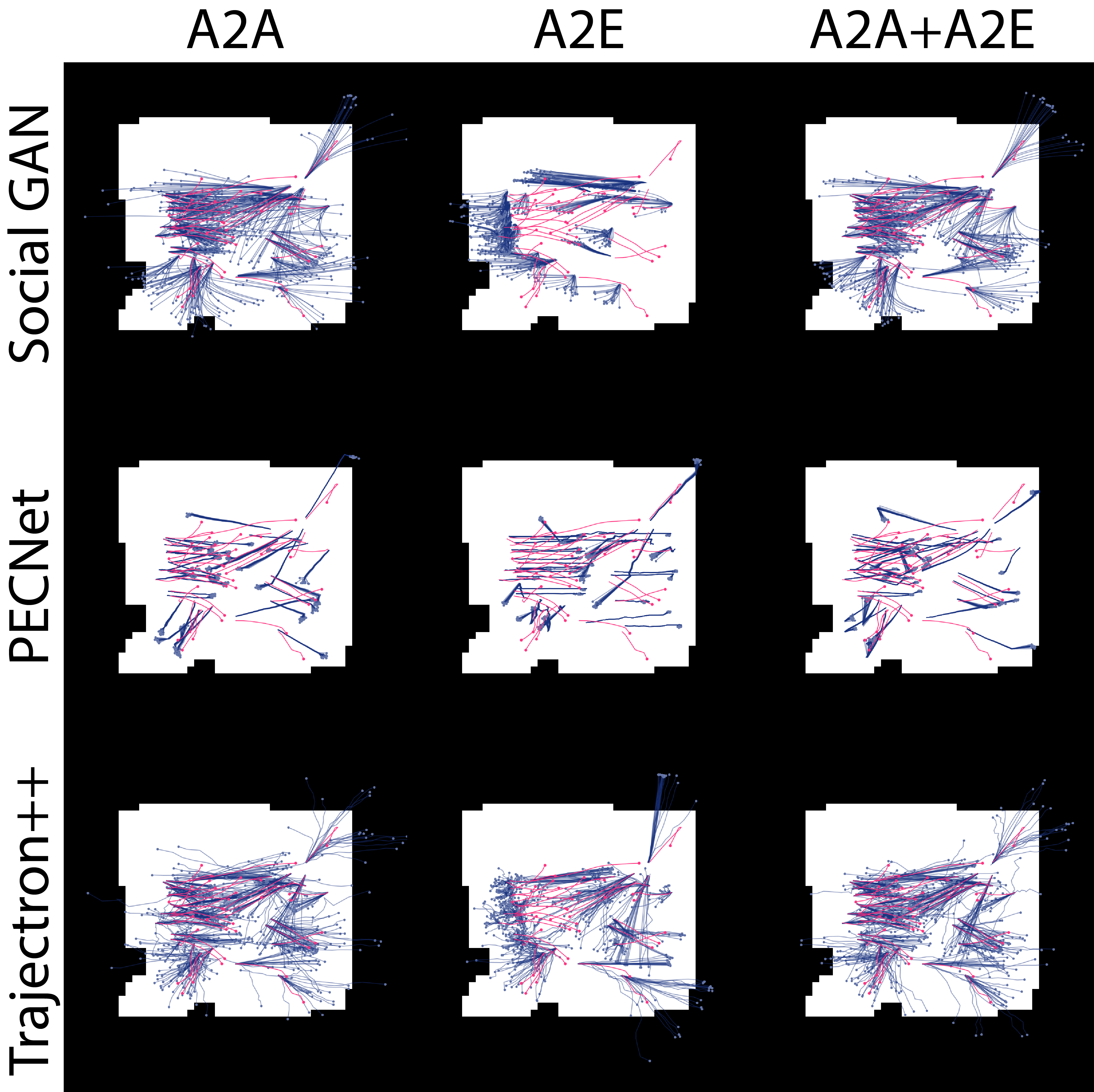The above table of images shows the predictions (blue) and ground truth (magenta) for 9 models tested on the same scenario. The model and training dataset for a particular image is given by the row and column it belongs to respectively.